▷ Diagonal matrix: definition, examples, properties, operations,...

On this post you will see what a diagonal matrix is and examples of diagonal matrices. Also, you will find how to operate with a diagonal matrix, and how to calculate its determinant and its inverse. In addition, we explain the properties and applications of this type of matrix. And, finally, you will find the explanations of a bidiagonal matrix and a tridiagonal matrix.

Table of Contents

What is a diagonal matrix?

The definition of diagonal matrix is as follows:

A diagonal matrix is a square matrix in which all the elements outside the main diagonal are zero (0). The entries on the main diagonal may or may not be null.

Examples of diagonal matrices

Once we know the meaning of diagonal matrix, we are going to see several examples of diagonal matrices tu fully understand the concept:

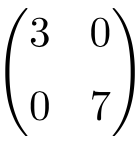
Example of 2×2 dimension diagonal matrix

example of a 2x2 dimension diagonal matrix

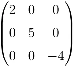
Example of 3×3 dimension diagonal matrix

example of a 3x3 dimension diagonal matrix

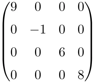
Example of 4×4 dimension diagonal matrix

example of a 4x4 dimension diagonal matrix

This type of matrix is usually written indicating the numbers on the diagonal:

$diag(2,5,1) = \left. \begin{pmatrix} 2 & 0 & 0 \\[1.1ex] 0 & 5 & 0 \\[1.1ex] 0 & 0 & 1 \end{pmatrix}$

Properties of diagonal matrices

Any diagonal matrix is also a symmetric matrix (see symmetric matrix definition).

A diagonal matrix is an upper and lower triangular matrix at the same time.

The identity matrix is a diagonal matrix:

$\begin{pmatrix} 1 & 0 & 0 \\[1.1ex] 0 & 1 & 0 \\[1.1ex] 0 & 0 & 1 \end{pmatrix}$

Similarly, the null matrix is also a diagonal matrix because all its elements that are not on the diagonal are zeros, although the numbers on the diagonal are 0.

$\begin{pmatrix} 0 & 0 & 0 \\[1.1ex] 0 & 0 & 0 \\[1.1ex] 0 & 0 & 0 \end{pmatrix}$

The eigenvalues of a diagonal matrix are the elements of its main diagonal.

$\begin{pmatrix} 7 & 0 & 0 \\[1.1ex] 0 & 3 & 0 \\[1.1ex] 0 & 0 & 4 \end{pmatrix} \longrightarrow \ \lambda = 3 \ ; \ \lambda = 4 \ ; \ \lambda = 7$

A square matrix is diagonal if and only if it is triangular and normal.

The adjoint (or adjugate) of a diagonal matrix is another diagonal matrix.

See: formula for adjoint of a matrix

Operations with diagonal matrices

One of the reasons that diagonal matrices are so important to linear algebra is the ease with which they allow you to perform calculations. That is why they are so used in mathematics.

Addition and subtraction of diagonal matrices

The addition (and subtraction) of two diagonal matrices is very simple: you just have to add (or subtract) the numbers of the diagonals.

$\displaystyle \text{diag}(a_1,... ,a_n) \pm \text{diag}(b_1 ,... , b_n) = \text{diag}(a_1\pm b_1,..., a_n\pm b_n)$

For example:

$\displaystyle \begin{pmatrix} 5 & 0 & 0 \\[1.1ex] 0 & -2 & 0 \\[1.1ex] 0 & 0 & 6 \end{pmatrix} +\begin{pmatrix} 1 & 0 & 0 \\[1.1ex] 0 & 3 & 0 \\[1.1ex] 0 & 0 & -4 \end{pmatrix} = \begin{pmatrix} 6& 0 & 0 \\[1.1ex] 0 & 1 & 0 \\[1.1ex] 0 & 0 & 2 \end{pmatrix}$

Multiplication of diagonal matrices

To solve a multiplication or a matrix product of two diagonal matrices we just have to multiply the elements of the diagonals with each other.

$\displaystyle \text{diag}(a_1,... ,a_n) \cdot \text{diag}(b_1 ,... , b_n) = \text{diag}(a_1\cdot b_1,..., a_n\cdot b_n)$

For example:

$\displaystyle \begin{pmatrix} 1 & 0 & 0 \\[1.1ex] 0 & -4 & 0 \\[1.1ex] 0 & 0 & -3 \end{pmatrix} \cdot\begin{pmatrix} 5 & 0 & 0 \\[1.1ex] 0 & -2 & 0 \\[1.1ex] 0 & 0 & 6 \end{pmatrix} = \begin{pmatrix} 5 & 0 & 0 \\[1.1ex] 0 & 8 & 0 \\[1.1ex] 0 & 0 & -18 \end{pmatrix}$

Power of a diagonal matrix

To calculate the power of a diagonal matrix we must raise each element of the diagonal to the exponent:

$\displaystyle A= \text{diag}(a_1,... ,a_n)$

$\displaystyle A^k= \text{diag}(a_1^k,... ,a_n^k)$

For example:

$\displaystyle\left. \begin{pmatrix} 3 & 0 & 0 \\[1.1ex] 0 & 2 & 0 \\[1.1ex] 0 & 0 & 4 \end{pmatrix}\right.^3= \begin{pmatrix} 27 & 0 & 0 \\[1.1ex] 0 & 8 & 0 \\[1.1ex] 0 & 0 & 64 \end{pmatrix}$

Determinant of a diagonal matrix

The determinant of a diagonal matrix is the product of the elements on the main diagonal.

$\displaystyle A= \text{diag}(a_1,... ,a_n)$

$\displaystyle \text{det}(A)= \prod_{i =1}^n a_i$

Look at the following solved exercise in which we find the determinant of a diagonal matrix by multiplying the elements on its main diagonal:

$\displaystyle \begin{vmatrix} 5 & 0 & 0 \\[1.1ex] 0 & 2 & 0 \\[1.1ex] 0 & 0 & 3 \end{vmatrix} = 5 \cdot 2 \cdot 3 = 30$

This theorem is easy to prove: we only have to calculate the determinant of a diagonal matrix by cofactors. This demonstration is detailed below using a generic diagonal matrix:

$\begin{aligned} \begin{vmatrix} a & 0 & 0 \\[1.1ex] 0 & b & 0 \\[1.1ex] 0 & 0 & c \end{vmatrix}& = a \cdot \begin{vmatrix} b & 0 \\[1.1ex] 0 & c \end{vmatrix} - 0 \cdot \begin{vmatrix} 0 & 0 \\[1.1ex] 0 & c \end{vmatrix} + 0 \cdot \begin{vmatrix} 0 & b \\[1.1ex] 0 & 0 \end{vmatrix} \\[2ex] & =a \cdot (b\cdot c) - 0 \cdot 0 + 0 \cdot 0 \\[2ex] & = a \cdot b \cdot c \end{aligned}$

Inverse of a diagonal matrix

A diagonal matrix is invertible if, and only if, all elements on the main diagonal are different from 0.

Also, the inverse of a diagonal matrix will always be another diagonal matrix with the reciprocals of the numbers on the main diagonal:

$\displaystyle A= \begin{pmatrix} 3 & 0 & 0 \\[1.1ex] 0 & 2 & 0 \\[1.1ex] 0 & 0 & 8 \end{pmatrix} \ \longrightarrow \ A^{-1}=\begin{pmatrix} \frac{1}{3} & 0 & 0 \\[1.1ex] 0 & \frac{1}{2} & 0 \\[1.1ex] 0 & 0 & \frac{1}{8} \end{pmatrix}$

From the previous characteristic, it can be deduced that the determinant of the inverse of a diagonal matrix is equal to the product of the reciprocals of the entries on the main diagonal:

$\displaystyle B= \begin{pmatrix} 2 & 0 & 0 \\[1.1ex] 0 & 4 & 0 \\[1.1ex] 0 & 0 & -1 \end{pmatrix}$

$\displaystyle\left| B^{-1}\right|=\cfrac{1}{2} \cdot \cfrac{1}{4} \cdot \cfrac{1}{-1}=-\cfrac{1}{8} = -0,125$

Applications of the diagonal matrix

As we have seen, solving calculations with diagonal matrices is very simple, since many zeros are involved in the operations. For that reason they are very useful in the field of mathematics.

For this same reason, so many studies have been made of how to diagonalize a matrix and, in fact, a method has even been reached for the diagonalization of matrices. See how to do the diagonalization of a matrix.

Thus, diagonalizable matrices are also quite relevant. Like the spectral decomposition theorem, which states the conditions for a matrix to be diagonalized.

Bidiagonal matrix

A bidiagonal matrix is a square matrix in which all elements that are not on the main diagonal or on the upper or lower diagonal are 0.

Upper bidiagonal matrix

$\begin{pmatrix} 3 & 2 & 0 \\[1.1ex] 0 & -5 & 1 \\[1.1ex] 0 & 0 & 6 \end{pmatrix}$

Lower bidiagonal matrix

$\begin{pmatrix} 1 & 0 & 0 \\[1.1ex] 6 & 2 & 0 \\[1.1ex] 0 & 7 & 4 \end{pmatrix}$

Tridiagonal matrix

A tridiagonal matrix is a square matrix whose only nonzero elements are those of the main diagonal and the adjacent diagonals above and below.

$\begin{pmatrix} 2 & 3 & 0 & 0 \\[1.1ex] -4 & 5 & 9 & 0 \\[1.1ex] 0 & 1 & 6 & -2 \\[1.1ex] 0 & 0 & 8 & 7 \end{pmatrix}$

Therefore, all diagonal, bidiagonal, and tridiagonal matrices are examples of band matrices. Since a band matrix has all its non-zero elements around the main diagonal.

What is a diagonal matrix?

Examples of diagonal matrices

Properties of diagonal matrices

Operations with diagonal matrices

Addition and subtraction of diagonal matrices

Multiplication of diagonal matrices

Power of a diagonal matrix

Determinant of a diagonal matrix

Inverse of a diagonal matrix

Applications of the diagonal matrix

Bidiagonal matrix

Tridiagonal matrix

Leave a Comment Cancel Reply