Solving systems of equations by Gaussian Elimination method

On this post you will learn what the Gaussian elimination method is and how to solve a system of equations by the Gaussian elimination method.

Table of Contents

What is the Gaussian elimination method?

The Gaussian elimination method, also called row reduction method, is an algorithm used to solve a system of linear equations with a matrix. The Gaussian elimination method consists of expressing a linear system in matrix form and applying elementary row operations to the matrix in order to find the value of the unknowns.

However, to understand how Gaussian elimination works, we must first know how to express a system of linear equations in matrix form and what row operations can be computed. So, we will explain these two things first, and then we will see how to apply Gaussian elimination method.

Augmented matrix of a system of linear equations

In linear algebra, a system of equations can be expressed in matrix form: the coefficients of the unknown x correspond to the first column of the matrix, the coefficients of the unknown y to the second column, the coefficients of the unknown z to the third column, and the constants to the fourth column.

For example:

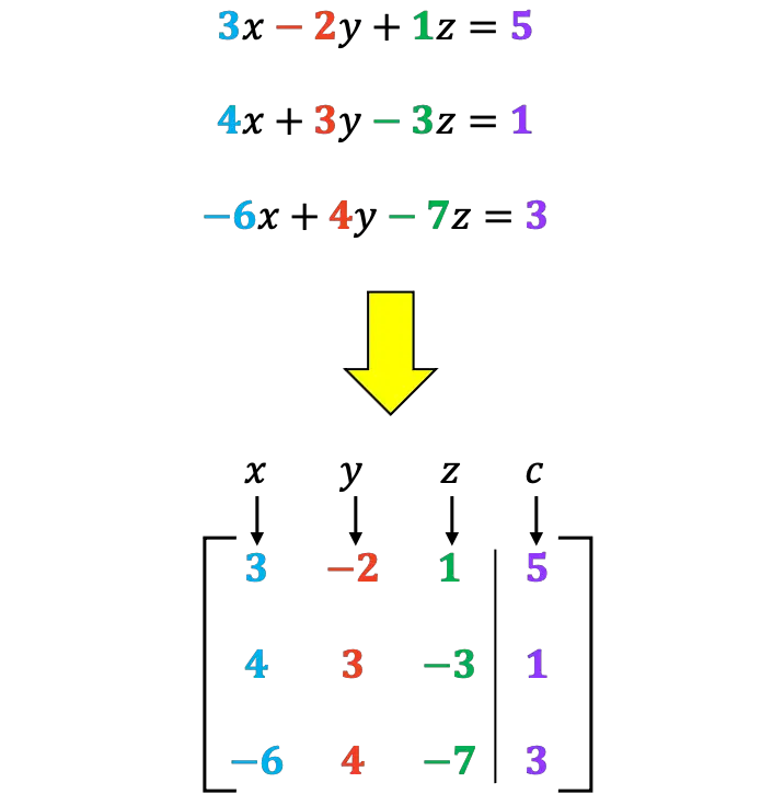
The matrix that represents the system of equations is called augmented matrix.

The objective of the Gaussian method is to convert the initial system of equations into a echelon system, that is, a system in which each equation has one less unknown than the previous one:

$\begin{array}{r} a_1x+b_1y+c_1z=d_1 \\[2ex] a_2x+b_2y+c_2z=d_2 \\[2ex] a_3x+b_3y+c_3z=d_3 \end{array} \ \color{orange}\bm{\longrightarrow}\color{black} \begin{array}{r} A_1x+B_1y+C_1z=D_1 \\[2ex] B_2y+C_2z=D_2 \\[2ex] C_3z=D_3 \end{array}$

In other words, we have to transform the augmented matrix into a matrix in row echelon form:

$\left[\begin{array}{ccc|c}a_1&b_1&c_1&d_1\\[1.1ex]a_2&b_2&c_2&d_2 \\[1.1ex] a_3&b_3&c_3&d_3 \end{array}\right] \ \color{orange}\bm{\longrightarrow}\color{black} \ \left[\begin{array}{ccc|c}A_1&B_1&C_1&D_1 \\[1.1ex] 0&B_2&C_2&D_2 \\[1.1ex] 0&0&C_3&D_3 \end{array}\right]$

To do this, we have to apply elementary operations on the rows of the matrix. So, let’s see what operations can be done in the Gaussian elimination method.

Elementary row operations

To convert the augmented matrix to a matrix in row echelon form, you can perform any of the following elementary operations:

Interchange two rows of the matrix.

For example, we can interchange rows 2 and 3 of a matrix:

$\left[\begin{array}{ccc|c}3&5&-2&1\\[2ex]-2&4&-1&2\\[2ex]6&1&-3&10\end{array}\right]\begin{array}{c}\\[2ex] \xrightarrow{R_2 \rightarrow R_3}\\[2ex]\xrightarrow{R_3 \rightarrow R_2}\end{array}\left[\begin{array}{ccc|c}3&5&-2&1\\[2ex]6&1&-3&10\\[2ex]-2&4&-1&2\end{array}\right]$

Multiply or divide all the terms in a row by a nonzero number.

For example, we can multiply the first row by 4, and divide the third row by 2:

$}\left[\begin{array}{ccc|c}1&-2&3&1\\[2ex]3&-1&5&-3\\[2ex]2&-4&-2&6\end{array}\right]\begin{array}{c}\xrightarrow{4R_1}\\[2ex]\\[2ex]\xrightarrow{R_3/2}\end{array}\left[\begin{array}{ccc|c}4&-8&12&4\\[2ex]3&-1&5&-3\\[2ex]1&-2&-1&3\end{array}\right]$

Add to a row another row multiplied by a scalar.

For example, in the following matrix we add row 3 multiplied by 1 to row 2:

$\left[\begin{array}{ccc|c}-1&-3&4&1\\[2ex]2&4&1&-5\\[2ex]1&-2&3&-1\end{array}\right]\begin{array}{c}\\[2ex]\xrightarrow{R_2+1\cdot R_3}\\[2ex]&\end{array}\left[\begin{array}{ccc|c}-1&-3&4&1\\[2ex]3&2&4&-6\\[2ex]1&-2&3&-1\end{array}\right]$

How to do Gaussian elimination

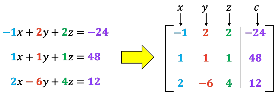
Now we are going to see with a solved example how to solve a system of linear equations using the Gaussian elimination method:

$\begin{array}{l}-x+2y+2z=-24 \\[2ex] x+y+z=48 \\[2ex] 2x-6y+4z=12\end{array}$

First of all, we find the augmented matrix of the system of equations:

As we will see later, it is better if the first number of the first row is 1. Therefore, we are going to change the order of rows 1 and 2:

$\left[\begin{array}{ccc|c} -1 & 2 & 2 &-24 \\[2ex] 1 & 1 & 1 & 48 \\[2ex] 2 & -6 & 4 & 12 \end{array} \right] \begin{array}{c} \xrightarrow{R_1 \rightarrow R_2} \\[2ex] \xrightarrow{R_2 \rightarrow R_1} \\[2ex] & \end{array} \left[\begin{array}{ccc|c} \color{blue}\boxed{\color{black}1} & 1 & 1 & 48 \\[2ex] -1 & 2 & 2 &-24 \\[2ex] 2 & -6 & 4 & 12 \end{array} \right]$

The goal of the Gaussian elimination method is to make the numbers below the main diagonal 0. So, we have to transform the red numbers to 0:

$\left[\begin{array}{ccc|c} 1 & 1 & 1 & 48 \\[2ex] \color{red}\bm{-1} & 2 & 2 &-24 \\[2ex] \color{red}\bm{2} & \color{red}\bm{-6} & 4 & 12 \end{array} \right]$

To eliminate these numbers we must do the appropriate elementary rows operations.

For example, the number -1, which is the first element in the second row, is the negative of 1, the first element in the first row. So if we add the first row to the second row, the -1 will be eliminated:

$\begin{array}{lccc|c} & -1 & 2 & 2 & -24 \\ + & \phantom{-}1 & 1 & 1 & \phantom{-}48 \\ \hline & \phantom{-}0 & 3 & 3 & \phantom{-}24 \end{array} \begin{array}{l} \color{blue}\bm{\leftarrow R_2} \\ \color{blue}\bm{\leftarrow R_1} \\ \phantom{hline} \\ \end{array}$

By adding the rows we obtain the following matrix:

$\left[\begin{array}{ccc|c} 1 & 1 & 1 & 48 \\[2ex] -1 & 2 & 2 & -24 \\[2ex] 2 & -6 & 4 & 12 \end{array}\right]\begin{array}{c} \\[2ex] \xrightarrow{R_2+R_1} \\[2ex] & \end{array} \left[\begin{array}{ccc|c} 1 & 1 & 1 & 48 \\[2ex] \color{blue}\boxed{\color{black}0} & 3 & 3 & 24 \\[2ex] 2 & -6 & 4 & 12 \end{array} \right]$

In this way we have transformed the -1 into a 0.

Now we are going to zero the number 2 out. To do so, we add the first row multiplied by -2 to the third row:

$\begin{array}{lccc|c} & \phantom{-}2 & -6 & \phantom{-}4 & \phantom{-}12 \\ + & -2 & -2 & -2 & -96 \\ \hline & \phantom{-}0 & -8 & \phantom{-}2 & -84 \end{array} \begin{array}{l} \color{blue} \bm{\leftarrow R_3} \\ \color{blue} \bm{\leftarrow -2 R_1} \\ \phantom{hline} \\ \end{array}$

And the following matrix is obtained:

$\left[\begin{array}{ccc|c} 1 & 1 & 1 & 48 \\[2ex] 0 & 3 & 3 & 24 \\[2ex] 2 & -6 & 4 & 12 \end{array} \right]\begin{array}{c} \\[2ex] \\[2ex] \xrightarrow{R_3-2R_1} \end{array} \left[\begin{array}{ccc|c} 1 & 1 & 1 & 48 \\[2ex] 0 & 3 & 3 & 24 \\[2ex] \color{blue}\boxed{\color{black}0} & -8 & 2 & -84 \end{array}\right]$

Now we have to convert the -8 to 0. To do this, we multiply the third row by 3 and add the second row multiplied by 8:

$\begin{array}{lccc|r} & 0 & -24 & \phantom{2}6 & -252 \\ + & 0 & \phantom{-}24 & 24 & \phantom{-}192 \\ \hline & 0 & \phantom{-2}0 & 30 & -60 \end{array} \begin{array}{l}\color{blue}\bm{ \leftarrow 3R_3} \\\color{blue}\bm{ \leftarrow 8R_2} \\ \phantom{hline} \\ \end{array}$

Therefore, we obtain the following matrix:

$\left[\begin{array}{ccc|c} 1 & 1 & 1 & 48 \\[2ex] 0 & 3 & 3 & 24 \\[2ex] 0 & -8 & 2 & -84 \end{array}\right]\begin{array}{c} \\[2ex] \\[2ex] \xrightarrow{3R_3+8R_2} \end{array} \left[\begin{array}{ccc|c} 1 & 1 & 1 & 48 \\[2ex] 0 & 3 & 3 & 24 \\[2ex] 0 & \color{blue}\boxed{\color{black}0} & 30 & -60 \end{array} \right]$

As you can see, with all these transformations we have made all the numbers below the main diagonal 0. That is, the matrix is in row echelon form (or triangular form).

Now we must transform the matrix into a system of equations with unknowns. For this, remember that the first column of the matrix corresponds to the unknown x, the second column to the unknown y, the third column to the unknown z, and the last column are the constants of the equations:

$\left[\begin{array}{ccc|c} 1 & 1 & 1 & 48 \\[2ex] 0 & 3 & 3 & 24 \\[2ex] 0 & 0 & 30 & -60 \end{array} \right] \ \longrightarrow \ \begin{array}{r} 1x+1y+1z=48 \\[2ex] 3y+3z=24 \\[2ex] 30z=-60 \end{array}$

And finally, to solve the system we have to find the values of the unknowns from the bottom up. Since the last equation only has one unknown, and therefore, we can easily find its value:

$30z = -60$

$z=-2$

Now we back-substitute into the second row to evaluate the unknown y:

$3y+3z=24 \ \xrightarrow{z \ = \ -2} \ 3y+3\cdot (-2)=24$

$3y-6=24$

$y=10$

And we do the same with the first equation of the system: we back-substitute the values of the other unknowns and solve for x:

$x+y+z=48 \ \xrightarrow{y \ = \ 10 \ ; \ z \ = \ -2} \ x+10-2=48$

$x=40$

Thus, the solution of the system of equations is:

$\bm{x=40} \qquad \bm{y=10} \qquad \bm{z=-2}$

We have solved the system of equations by transforming the augmented matrix into a matrix in echelon form. However, there are authors who prefer to continue applying row operations until the matrix is in reduced row echelon form (zeros above and below the main diagonal), in this case, the process is called Gauss-Jordan elimination.

Gaussian elimination method

What is the Gaussian elimination method?

Augmented matrix of a system of linear equations

Elementary row operations

How to do Gaussian elimination

2 thoughts on “Gaussian elimination method”

Leave a Comment Cancel Reply