What is an Orthogonal Matrix? (examples, properties, formula,...)

On this post you will see what orthogonal matrices are and their relation with the inverse of a matrix. You will also see several examples and the formula that verifies every orthogonal matrix, with which you will know how to find one quickly. Finally, you will find the properties and applications of these peculiar matrices together with a typical solved exam exercise.

Table of Contents

What is an orthogonal matrix?

The definition of orthogonal matrix is as follows:

An orthogonal matrix is a square matrix with real numbers that multiplied by its transpose is equal to the Identity matrix. That is, the following condition is met:

$A \cdot A^T = A^T \cdot A = I$

Where A is an orthogonal matrix and A^T is its transpose.

For this condition to be fulfilled, the columns and rows of an orthogonal matrix must be orthogonal unit vectors, in other words, they must form an orthonormal basis. That is why some mathematicians also call them orthonormal matrices.

Inverse of an orthogonal matrix

Another way to explain the concept of an orthogonal matrix is by means of the inverse matrix, because the transpose of an orthogonal matrix is equal to its inverse.

To fully understand this theorem, it is important to know how to invert a matrix. On this link you will find a detailed explanation of the inverse of a matrix, all its properties, and step by step solved exercises.

It is easy to prove that the inverse of an orthogonal matrix is equivalent to its transpose using the orthogonal matrix condition and the main property of inverse matrices:

$\left.\begin{array}{c} A \cdot A^T =I \\[2ex] A \cdot A^{-1} = I\end{array} \right\} \longrightarrow \ A^T=A^{-1}$

Thus, an orthogonal matrix will always be an invertible or non-degenerate matrix. See properties of invertible matrix.

Examples of orthogonal matrices

Next we are going to see several examples of orthogonal matrices to fully understand its meaning.

Example of a 2×2 orthogonal matrix

The following matrix is a 2×2 dimension orthogonal matrix:

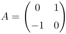
We can check that it is orthogonal by calculating the product by its transpose:

$\displaystyle A \cdot A^T$

$\displaystyle A\cdot A^T= \begin{pmatrix} 0 & 1 \\[1.1ex] -1 & 0 \end{pmatrix} \cdot \begin{pmatrix} 0 & -1 \\[1.1ex] 1 & 0 \end{pmatrix} = \begin{pmatrix} 1 & 0 \\[1.1ex] 0 & 1 \end{pmatrix}$

As the result gives the unit matrix, it is checked that A is an orthogonal matrix.

Example of a 3×3 orthogonal matrix

The following matrix is an orthogonal matrix of order 3:

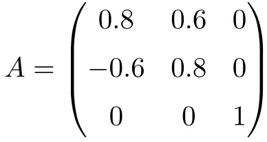
It can be shown that it is orthogonal by multiplying matrix A by its transpose:

$\displaystyle A\cdot A^T = \begin{pmatrix}0.8&0.6&0\\[1.1ex] -0.6&0.8&0\\[1.1ex] 0&0&1\end{pmatrix}\cdot \begin{pmatrix}0.8&-0.6&0\\[1.1ex] 0.6&0.8&0\\[1.1ex] 0&0&1\end{pmatrix}= \begin{pmatrix} 1 & 0 & 0\\[1.1ex] 0 & 1 & 0 \\[1.1ex] 0&0&1\end{pmatrix}$

The product results in the Identity matrix, therefore, A is an orthogonal matrix.

Formula to find a 2×2 orthogonal matrix

Now we are going to see the proof that all orthogonal matrices of order 2 follow the same pattern, furthermore, we are going to deduce how to find a 2×2 orthogonal matrix with a simple formula.

Let A be a generic 2×2 matrix:

$\displaystyle A=\begin{pmatrix} a & b \\[1.1ex] c & d \end{pmatrix}$

For this matrix to be orthogonal, the following matrix equation must be satisfied:

$\displaystyle A \cdot A^T = I$

$\displaystyle \begin{pmatrix} a & b \\[1.1ex] c & d \end{pmatrix} \cdot \begin{pmatrix} a & c \\[1.1ex] b & d \end{pmatrix} =\begin{pmatrix} 1 & 0 \\[1.1ex] 0 & 1 \end{pmatrix}$

Solving the matrix multiplication we obtain the following equations:

$\displaystyle \begin{pmatrix} a^2+b^2 & ac+bd \\[1.1ex] ac+bd & c^2+d^2 \end{pmatrix}=\begin{pmatrix} 1 & 0 \\[1.1ex] 0 & 1 \end{pmatrix}$

$\displaystyle \begin{array}{c}a^2+b^2=1 \\[2ex] ac+bd=0 \\[2ex] c^2+d^2=1 \end{array} \qquad \begin{array}{l} (1) \\[2ex] (2) \\[2ex] (3) \end{array}$

If we look closely, these equalities are very similar to the fundamental Pythagorean trigonometric identity:

$\displaystyle \sin ^2\alpha+\cos ^2\alpha=1$

Therefore, the terms that satisfy equations (1) and (3) are:

$\displaystyle \begin{array}{l} a = \cos \theta \qquad \qquad \qquad c = \sin\phi \\[2ex] b = \sin \theta \qquad \qquad \qquad d = \cos \phi\end{array}$

In addition, substituting the values in the second equation we obtain the relation between both angles:

$\displaystyle ac+bd=0$

$\displaystyle \cos\theta\sin\phi+\sin\theta\cos\phi=0$

$\displaystyle \tan\phi=-\tan\theta$

That is, one of the following two conditions must be met:

$\displaystyle \text{if} \quad c=\sin\phi=-\sin\theta \quad \longrightarrow \quad d=\cos\phi=\cos\theta$

$\displaystyle \text{if} \quad d=\cos \phi=-\cos \theta \quad \longrightarrow \quad c=\sin\phi=\sin\theta$

So, in conclusion, orthogonal matrices must have the structure of one of the following two matrices:

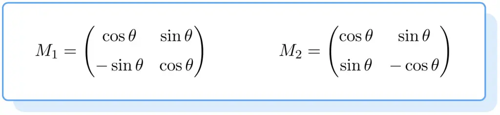
Where $\theta$ is a real number.

In fact, if as an example we give the value of $\displaystyle \theta = \frac{ pi}{2}$ and take the first matrix form, we will obtain the matrix that we have checked to be orthogonal above in the section “Example of a 2×2 orthogonal matrix”:

$\displaystyle M_1 \left(\theta =\frac{\pi}{2}\right)=\begin{pmatrix} \cos \cfrac{\pi}{2} &\sin \cfrac{\pi}{2} \\[4ex] -\sin \cfrac{\pi}{2} & \cos \cfrac{\pi}{2} \end{pmatrix}=\begin{pmatrix} \vphantom{\frac{\pi}{2}}0 &1 \\[2ex]\vphantom{\frac{\pi}{2}} -1 & 0 \end{pmatrix}$

Properties of an orthogonal matrix

The characteristics of this type of matrix are:

An orthogonal matrix can never be a singular matrix, since it can always be inverted. In this regard, the inverse of an orthogonal matrix is another orthogonal matrix.

Any orthogonal matrix can be diagonalized. So, orthogonal matrices are orthogonally diagonalizable.

See: how to perform matrix diagonalization.

All the eigenvalues of an orthogonal matrix have modulus 1.

See: how to calculate the eigenvalues of a matrix.

Any orthogonal matrix with only real numbers is also a normal matrix.

The analog of the orthogonal matrix in a complex number field is the unitary matrix.

Obviously, the identity matrix is an orthogonal matrix.

See definition of identity matrix.

The set of orthogonal matrices of dimension n×n together with the operation of the matrix product is a group called the orthogonal group. That is, the product of two orthogonal matrices is equal to another orthogonal matrix.

Furthermore, the result of multiplying an orthogonal matrix by its transpose can be expressed using the Kronecker delta:

$\displaystyle \left(A\cdot A^{T}\right)_{ij} = \delta_{ij}=\begin{cases}1 & \mbox{si }i = j, \\[2ex] 0 & \mbox{si }i \ne j\end{cases}$

Finally, the determinant of an orthogonal matrix is always equal to +1 or -1.

$\displaystyle \text{det}(A) = \pm 1$

Solved exercise of orthogonal matrices

Next we are going to solve an exercise of orthogonal matrices.

Given the following square matrix of order 3, find the values of $a$ and $b$ so that the matrix is orthogonal:

$\displaystyle A=\frac{1}{3}\begin{pmatrix}a&a&1\\[1.1ex] b&1&b\\[1.1ex] 1&a&a\end{pmatrix}$

In order to satisfy the orthogonality of the matrix, the product of the matrix and its transpose must be equal to the identity matrix. Thus:

$\displaystyle A\cdot A^T = I$

$\displaystyle \frac{1}{3}\begin{pmatrix}a&a&1\\[1.1ex] b&1&b\\[1.1ex] 1&a&a\end{pmatrix} \cdot \frac{1}{3}\begin{pmatrix}a&b&1\\[1.1ex] a&1&a\\[1.1ex] 1&b&a\end{pmatrix}=\begin{pmatrix}1&0&0\\[1.1ex] 0&1&0\\[1.1ex] 0&0&1\end{pmatrix}$

We solve the matrix multiplication:

$\displaystyle \frac{1}{9}\begin{pmatrix}2a^2+1&ab+a+b&2a+a^2\\[1.5ex] ab+a+b&2b^2+1&b+a+ab\\[1.5ex] 2a+a^2&b+a+ab&1+2a^2\end{pmatrix} =\begin{pmatrix}1&0&0\\[1.5ex] 0&1&0\\[1.5ex] 0&0&1\end{pmatrix}$

We can get an equation for the upper left corner of the matrices, because the elements located in that position have to coincide. So:

$\displaystyle \frac{1}{9}(2a^2+1) = 1$

We solve the equation:

$\displaystyle 2a^2+1 = 9$

$\displaystyle 2a^2 = 8$

$\displaystyle a^2 = 4$

$\displaystyle \bm{a = \pm 2}$

However, there are equations that do not hold for the positive solution, for example the one in the upper right corner. So only the negative solution is feasible.

On the other hand, to calculate the variable $b$ we can match, for example, the terms placed in the second row of the first column:

$\displaystyle \frac{1}{9}(ab+a+b) = 0$

$\displaystyle ab+a+b = 0$

Substituting the value of $a$ in the equation:

$\displaystyle -2b-2+b = 0$

$\displaystyle -b =2$

$\displaystyle \bm{b =-2}$

Ultimately, the only possible solution is:

$\displaystyle \bm{a = b = -2}$

So the orthogonal matrix that has those values is:

$\displaystyle A=\frac{1}{3}\begin{pmatrix}-2&-2&1\\[1.1ex] -2&1&-2\\[1.1ex] 1&-2&-2\end{pmatrix}$

Applications of orthogonal matrices

Although it may not seem like it, orthogonal matrices are very important in mathematics, especially in the field of linear algebra.

In geometry, orthogonal matrices represent isometric transformations that do not modify distances and angles in real vector spaces, for that reason they are called orthogonal transformations. Furthermore, these transformations are internal isomorphisms of such vector space. These transformations can be rotations, specular reflections, or inversions.

Finally, this type of matrix is also used in physics, since it allows studying the motion of rigid bodies. And they are even used in the formulation of certain field theories.

Orthogonal matrix